Hartley Oscillator

The Hartley oscillator is a type of LC (Inductance-Capacitance) oscillator commonly used in radio receivers. It is designed to generate sinusoidal oscillations at RF (Radio Frequency) levels. The unique feature of the Hartley oscillator is its center-tapped inductor, which allows the circuit to produce a sinusoidal output waveform. The center tap provides the necessary phase shift for continuous oscillation by enabling feedback to flow from the inductor's center to the amplifier. The frequency of oscillations in a Hartley oscillator can be adjusted by changing the values of the inductance and capacitance, which are the key factors controlling the oscillation frequency.

Key Factors of the Hartley Oscillator:

• External Temperature
• Component Quality
• Uniformity

Factors Affecting the Hartley Oscillator:

Changes in temperature or over time can cause the values of electronic components to drift, which may alter the oscillator's frequency. To mitigate this, low temperature coefficient components are often used in high-precision applications.

Working of the Hartley Oscillator

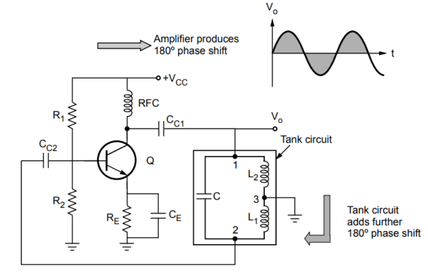
The figure below shows the practical circuit of a Hartley oscillator using a BJT (Bipolar Junction Transistor) as the active device. The resistors $R_1$, $R_2$, and $R_E$ are used for biasing.

• The RFC (Radio Frequency Choke) has a high reactance value at high frequencies and can be considered an open circuit. However, for DC operation, it acts as a short circuit, thus not interfering with the DC operation.

• The RFC ensures isolation between AC and DC operations. The capacitors $C_{C1}$ and $C_{C2}$ are coupling capacitors, while $C_E$ is the emitter bypass capacitor. The amplifier provides a 180° phase shift.

• In the feedback circuit, because the center of the inductors $L_1$ and $L_2$ is grounded, an additional 180° phase shift is provided, satisfying the Barkhausen condition. In this oscillator:

  $X_1 = \omega L_1$, $X_2 = \omega L_2$, $X_3 = -\frac{1}{\omega C}$.

• For an LC oscillator, $X_1 + X_2 + X_3 = 0$.

  $\omega L_1 + \omega L_2 - \frac{1}{\omega C} = 0$

  $\omega(L_1 + L_2) = \frac{1}{\omega C}$

  $\omega = \frac{1}{\sqrt{(L_1 + L_2)C}}$

  $f = \frac{1}{2\pi\sqrt{(L_1 + L_2)C}}$

• The inductance $L_1 + L_2$ is the equivalent inductance, denoted as $L_{eq}$. The $H_{fe}$ of the BJT must be $\frac{L_1}{L_2}$.

  $H_{fe} = \frac{L_1}{L_2}$

• In practice, $L_1$ and $L_2$ are often wound on a single core, resulting in mutual inductance $M$ between them.

  $L_{eq} = L_1 + L_2 + 2M$

  $f = \frac{1}{2\pi\sqrt{L_{eq} C}}$

  $H_{fe} = \frac{L_1 + M}{L_2 + M}$

Derivation of Frequency of Oscillations

• The output current is the collector current, which is $h_{fe} I_b$, where $I_b$ is the base current. Assuming the coupling capacitors are shorted, the capacitor $C$ is connected between the collector and base.

• With the emitter grounded for AC analysis, $L_1$ is between the emitter and base, while $L_2$ is between the emitter and collector. The equivalent circuit is shown below.

  

• $h_{ie}$ is the input impedance of the transistor. The output current is $I_b$, while the input current is $h_{fe} I_b$. The current source can be converted to a voltage source as shown below.

  

$V_0 = h_{fe} I_b j X_{L2} = h_{fe} I_b j \omega L_2$

• The total current $I$ is:

  $I = \frac{-V_0}{\left[X_{L2} + X_C\right] + \left[X_{L1} \parallel h_{ie}\right]} \quad \text{(i)}$

• The negative sign indicates that the direction of $I$ is opposite to the polarity of $V_0$.

  $X_{L2} + X_C = j \omega L_2 + \frac{1}{j \omega C} = \frac{-\omega^2 L_2 C + 1}{j \omega C}$

  $X_{L1} \parallel h_{ie} = \frac{j \omega L_1 \cdot h_{ie}}{j \omega L_1 + h_{ie}}$

  $I = \frac{-h_{fe} I_b j \omega L_2}{\frac{-\omega^2 L_2 C + 1}{j \omega C} + \frac{j \omega L_1 \cdot h_{ie}}{j \omega L_1 + h_{ie}}}$

Using the current division rule for parallel elements:

$I_b = I \times \frac{j \omega L_1}{j \omega L_1 + h_{ie}}$

$I_b = \frac{-h_{fe} I_b j \omega L_2}{\frac{-\omega^2 L_2 C + 1}{j \omega C} + \frac{j \omega L_1 \cdot h_{ie}}{j \omega L_1 + h_{ie}}} \times \frac{j \omega L_1}{j \omega L_1 + h_{ie}}$

$1 = \frac{j \omega^3 h_{fe} C L_1 L_2}{\left[h_{ie} - \omega^2 C h_{ie} (L_1 + L_2)\right] + j \omega L_1 \left(1 - \omega^2 L_2 C\right)}$

• Rationalizing the right-hand side of the above equation:

  $1 = \frac{\omega^4 h_{fe} L_1^2 L_2 C (1 - \omega^2 L_2 C)}{[h_{ie} - \omega^2 C h_{ie} (L_1 + L_2)]^2 + \omega^2 L_2^2 C^2} +$

  $\frac{ j \omega^3 h_{fe} L_1 L_2 C [h_{ie} - \omega^2 C h_{ie} (L_1 + L_2)]}{[h_{ie} - \omega^2 C h_{ie} (L_1 + L_2)]^2 + \omega^2 L_2^2 C^2}$

  $\quad \text{(ii)}$

• The imaginary part of the right-hand side must be zero.

  $\omega^3 h_{fe} L_1 L_2 C \cdot$ $\left[h_{ie} - \omega^2 C h_{ie} (L_1 + L_2)\right] = 0$

  $1 - \omega^2 C (L_1 + L_2) = 0 \quad \text{i.e.} \quad \omega = \frac{1}{\sqrt{C(L_1 + L_2)}}$

  $f = \frac{1}{2\pi\sqrt{C(L_1 + L_2)}} = \frac{1}{2\pi\sqrt{C(L_{eq})}} \quad \text{(iii)}$

• Equating the magnitudes of both sides of equation (ii) and using $\omega = \frac{1}{\sqrt{C(L_1 + L_2)}}$, we get:

  $h_{fe} = \frac{L_1}{L_2} \quad \text{(iv)}$

In practice, $L_1$ and $L_2$ may be wound on a single core so that there exists a mutual inductance between them, denoted as $M$.

• In such a case, the mutual inductance is considered when determining the equivalent inductance $L_{eq}$. Hence,

  $L_{eq} = L_1 + L_2 + 2M$

• If $L_1$ and $L_2$ are assisting each other, the sign of $2M$ is positive, while if $L_1$ and $L_2$ are in series opposition, the sign of $2M$ is negative.

• The expression for the frequency of the oscillations remains the same as given by equation (iii).

Advantages

1. The frequency can be easily varied by a variable capacitor.

2. The output amplitude remains constant over the frequency range.

3. The feedback ratio of $L_1$ to $L_2$ remains constant.

Disadvantages

1. The output is rich in harmonics, hence not suitable for pure sine wave requirements.

2. Poor frequency stability.

Applications

1. Used as a local oscillator in TV and radio receivers.

2. In function generators.

3. In radio frequency sources.