Colpitts Oscillator

The Colpitts oscillator is similar to the Hartley oscillator, but it uses a different arrangement for the tank circuit components. Instead of using inductors and capacitors in the same configuration as the Hartley oscillator, the Colpitts oscillator swaps their roles.

Working of the Colpitts Oscillator

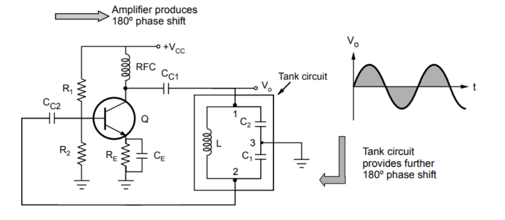
The figure below shows a Colpitts oscillator using a BJT amplifier stage.

In this circuit, the amplifier stage uses a BJT in a common emitter configuration to provide a $180^\circ$ phase shift. The resistors $R_1$, $R_2$, and $R_E$ are biasing resistors.

• The RFC (radio frequency choke) provides isolation between AC and DC operations. The capacitors $C_{C1}$ and $C_{C2}$ are coupling capacitors. In the feedback circuit, the center tap of $C_1$ and $C_2$ is grounded, providing an additional $180^\circ$ phase shift, which satisfies the Barkhausen criterion.

• In this oscillator:

  • $X_1 = -\frac{1}{\omega C_1}$
  • $X_2 = -\frac{1}{\omega C_2}$
  • $X_3 = \omega L$

• For the LC oscillator, the condition is:

  $\quad X_1 + X_2 + X_3 = 0$

  $\therefore \; \; \; \; \; \; \; -\frac{1}{\omega C_1} - \frac{1}{\omega C_2} + \omega L = 0$

  $\quad \text{i.e.} \quad \omega L = \frac{1}{\omega} \left[\frac{1}{C_1} + \frac{1}{C_2}\right]$

  $\therefore \; \; \; \; \; \; \; \omega^2 = \frac{1}{L} \left[\frac{C_1 C_2}{C_1 + C_2}\right]$

  $\quad \text{where} \quad \frac{C_1 C_2}{C_1 + C_2} = C_\text{eq}$

  $\therefore \; \; \; \; \; \; \; \omega = \frac{1}{\sqrt{L C_\text{eq}}} \quad \text{i.e.} \quad f = \frac{1}{2\pi \sqrt{L C_\text{eq}}}$

  $\text{where} \quad C_\text{eq} = \frac{C_1 C_2}{C_1 + C_2}$

To satisfy the magnitude condition of the Barkhausen criterion, the $h_{fe}$ of the BJT used is:

$h_{fe} = \frac{C_2}{C_1}$

Derivation of Frequency of Oscillations

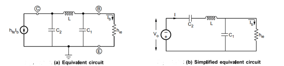
The equivalent circuit and simplified equivalent circuit are shown below.

In the simplified equivalent circuit:

$V_0 = h_\text{fe} I_b X_{C2} = \frac{-j h_\text{fe} I_b}{\omega C_2}$

• $X_{C2} = \frac{1}{j \omega C_2} = \frac{-j}{\omega C_2}$

• The total current $I$ is:

  $I = \frac{-V_0}{[X_{C2} + X_L] + [X_{C1} \parallel h_{ie}]}$

  $X_{C2} + X_L = \frac{-j}{\omega C_2} + j \omega L = \frac{-j (1 - \omega^2 L C_2)}{\omega C_2}$

  $X_{C1} \parallel h_{ie} = \frac{\frac{-j}{\omega C_1} \cdot h_{ie}}{\frac{-j}{\omega C_1} + h_{ie}}$

  $\therefore \; \; \; \; \; \; I = \frac{\frac{-j h_\text{fe} I_b}{\omega C_2}}{\frac{-j (1 - \omega^2 L C_2)}{\omega C_2} + \frac{j h_{ie}}{\frac{-j}{\omega C_1} + h_{ie}}}$

Using the current division rule for parallel elements:

$I_b = I \times \frac{\frac{-j}{\omega C_1}}{\frac{-j}{\omega C_1} + h_{ie}} = \frac{-j I}{\frac{-j + \omega C_1 h_{ie}}{\omega C_1}}$

$\therefore \; \; \; \; \; \; I_b = \frac{-j \left[\frac{j h_\text{fe} I_b}{\omega C_2}\right]}{\frac{-j (1 - \omega^2 L C_2)}{\omega C_2}} \times \frac{-j h_{ie}}{\frac{-j}{\omega C_1} + h_{ie}}$

$\therefore \; \; \; \; \; \; 1 = \frac{-h_\text{fe}}{(1 - \omega^2 L C_2) + j \omega h_{ie} [C_1 C_2 - \omega^2 L C_1 C_2]} \quad \text{(i)}$

To have the imaginary part of the above equation equal to zero:

$C_1 + C_2 - \omega^2 L C_1 C_2 = 0$

$\text{i.e.} \quad \omega^2 = \frac{C_1 + C_2}{L C_1 C_2} = \frac{1}{L \left[\frac{C_1 C_2}{C_1 + C_2}\right]}$

$\therefore \; \; \; \; \; \; \omega = \frac{1}{\sqrt{L C_\text{eq}}} \quad \text{and} \quad f = \frac{1}{2\pi \sqrt{L C_\text{eq}}}$

Substituting this result for $\omega$ into equation (i) for $h_{fe}$ and equating magnitudes of both sides:

$h_{fe} = \frac{C_2}{C_1}$

Advantages

• The Colpitts oscillator can generate sinusoidal signals of very high frequencies.
• It has good temperature stability.
• Frequency stability is high.
• The frequency can be varied using both variable capacitors.
• Fewer components are required.
• The amplitude of the output remains constant over a fixed frequency range.

Disadvantages

• Adjusting the feedback can be challenging.
• It has relatively poor isolation.

Applications

• The Colpitts oscillator is used as a high-frequency sine wave generator.
• It can be used as a temperature sensor with additional circuitry.
• Commonly used as a local oscillator in radio receivers.
• Used as an RF oscillator.
• Applied in mobile communications and other commercial applications.