Concepts of Production Function
Production generally refers to the process of transforming raw materials into finished goods. In economics, production is defined as the creation of goods both material and immaterial intended for sale in the market.
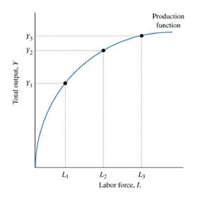
The production function expresses the relationship between the physical inputs and output of a firm for a given state of technology. It is a purely technical relation that connects factor inputs and outputs.
The production function can be mathematically represented as follows:
Qx = A . f(F1, F2, F3...........Fn)
Where:
- ( A ) is the efficiency parameter reflecting changes in technology. If technology improves, the value of ( A ) increases, allowing the producer to generate more output with the same amount of inputs.
- ( Qx ) represents the quantity of commodity (x).
- ( F1, F2, F3.......... Fn ) are the different factor inputs.
This equation indicates that the output of (x) depends on the factors ( F1, F2, F3, ..... Fn ), establishing a functional relationship between factor inputs and the quantity of good(x).
Types of Production Functions
Before analyzing the types of production functions, it is useful to understand the following terms:
-
Short-Run Production Functions Short-run production functions show the relationship between production and factors of production over a limited period. In the short run, not all factors may be available, and these factors can be divided into two types:
-
Fixed Factors
Fixed factors are those that cannot be changed in the short run and are kept constant. Examples include land, buildings, and machinery. -
Variable Factors
Variable factors are those that can be adjusted to change output in the short run. Examples include capital, labor, and raw materials.
-
-
Long-Run Production Functions Long-run production functions explain the relationship between production and factors of production over an extended period. This is also known as the law of returns to scale. In the long run, all factors of production are considered variable, meaning that firms can adjust all inputs to optimize production. his classification of fixed and variable factors is relevant only in the short run, while in the long run, all factors can be varied.
Returns to a Factor
Commonly referred to as factor productivity, returns to a factor describe the short-term relationship between output and input. The productivity from a single production unit is equivalent to the output generated, calculated under the assumption that all other factors remain constant.
Concept of Returns to a Factor
Returns to a factor relate to the overall behavior of total output when only one variable input is altered. This concept is primarily short-term and consists of three categories:
- Constant Returns to a Factor: Output increases proportionately with an increase in input.
- Increasing Returns to a Factor: Output increases at an increasing rate with more input.
- Diminishing Returns to a Factor: Output increases at a decreasing rate as more input is added.
Key Measures of Productivity
- Total Productivity: The total physical product generated at various levels of a specific input.
- Marginal Productivity: The additional output generated by adding one more unit of input while keeping all other inputs constant.
Law of Diminishing Marginal Productivity: The law of diminishing marginal productivity states that if one factor of production is increased while others remain unchanged, the additional output produced will eventually decline. Initially, productivity may rise with added input, but it will eventually decrease and can even become negative if too much input is added.
Significance of the Law
The law of diminishing returns is crucial in optimizing resource allocation and understanding production efficiency. It has implications in various fields, including economics and mathematical optimization.
Impact of Demand and Supply Changes
-
Changes in Demand
Several factors can cause demand for a product to change, including:
- Value of essential commodities
- Price forecasts
- Availability of substitutes
- Per capita income
- Population trends
- Consumer preferences
Effects of Demand Changes:
- Increase in Demand: If supply remains constant and demand rises, the demand curve shifts right, leading to higher equilibrium prices and increased competition among producers.
- Decrease in Demand: If demand falls while supply is constant, the demand curve shifts left, resulting in excess supply and increased competition.
-
Changes in Supply
Supply can change due to factors such as:
- Future price expectations
- Technological advancements
- Production costs
- Number of suppliers
- Competitive product costs
- Corporate goals
- Taxes
Effects of Supply Changes:
- Increase in Supply: If demand remains constant and supply increases, the supply curve shifts right, leading to lower equilibrium prices and heightened market competition.
- Decrease in Supply: If demand is constant but supply decreases, the supply curve shifts left, increasing demand at the equilibrium level.
Complex Market Scenarios
Several real-world situations can complicate the supply-demand relationship, including:
- Decreased demand with decreased supply
- Increased supply with decreased demand
- Increased demand with increased supply
- Decreased supply with increased demand
Returns to a scale
The term returns to scale refers to changes in output as all factors are varied by the same proportion. — Koutsoyiannis
Returns to scale relates to the behavior of total output when all inputs are adjusted, and it is a long-run concept. — Leibhafsky
Law of Returns to Scale in Production
The law of returns to scale illustrates the relationship between inputs and outputs over the long term. When all factors of production are adjusted simultaneously by the same proportion, we refer to this change in quantity as a scale change. For instance, if all factors of production are doubled or tripled, we are moving toward large-scale production. Conversely, halving or reducing them to one-third signifies small-scale production. The change in output resulting from these changes in input is termed returns to scale.
Explanation of the Law
According to the law, when all inputs are increased in the same proportions, the resulting output may not increase proportionately. Changes in output can be categorized into three stages:
- Increasing Returns to Scale
- Constant Returns to Scale
- Diminishing Returns to Scale
Table of Production Scale
| Scale of Production | Inputs (Land + Labor) | Total Productivity | Marginal Productivity |
|---|---|---|---|
| A | 1 + 2 | 4 | 4 |
| B | 2 + 4 | 10 | 6 |
| C | 3 + 6 | 18 | 8 |
| D | 4 + 8 | 28 | 10 |
| E | 5 + 10 | 38 | 10 |
| F | 6 + 12 | 48 | 10 |
| G | 7 + 14 | 56 | 8 |
| H | 8 + 16 | 62 | 6 |
| I | 9 + 16 | 66 | 4 |
In this table, all inputs are altered by equal quantities. The changes in output are evident from total and marginal returns. Initially, when inputs are doubled, marginal returns increase more than proportionately—this is called increasing returns. In subsequent combinations, output increases proportionately, indicating constant returns. Eventually, as inputs continue to rise, diminishing returns set in.
Diagrammatic Explanation
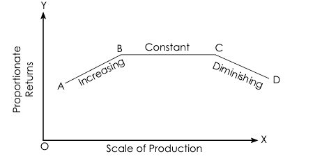
In this diagram, the scale of inputs is plotted along the X-axis and marginal returns along the Y-axis. Initially, as inputs increase, the marginal returns curve rises, reflecting increasing returns. The curve stabilizes, indicating constant returns, and eventually, further increases in input lead to diminishing returns.
Increasing Returns to Scale
When the proportional increase in output exceeds the proportional increase in inputs, this is known as increasing returns to scale. For example, if inputs are doubled, output more than doubles.
Causes of Increasing Returns:
- Specialization or division of labor
- Indivisible factors
- Economies of scale
- Volume discounts
Constant Returns to Scale
If the proportional increase in output matches the proportional increase in inputs, we have constant returns to scale. Here, doubling the inputs results in exactly double the output. There are no specific causes for constant returns; it simply indicates the transition from increasing to diminishing returns.
Diminishing Returns to Scale
When the proportional increase in output is less than the proportional increase in inputs, it is termed diminishing returns to scale. For instance, if inputs are doubled, output increases by less than double.
Causes of Diminishing Returns:
- Management challenges
- Limitations of human factors
- Lack of cooperation and coordination
- Rising prices of inputs
Here's a clear difference table comparing Returns to a Variable Factor and Returns to Scale:
| Aspect | Returns to a Variable Factor | Returns to Scale |
|---|---|---|
| Time Frame | Operates in the short run | Operates in the long run |
| Input Variation | Only the quantity of a variable factor is varied | All factor inputs are varied in the same proportion |
| Factor Proportion Change | There is a change in the factor proportion. For example, if 1 unit of labor is added to 1 acre of land, the land-labor ratio changes from 1:1 to 1:2. | There is no change in factor ratios. For example, if a firm employs 1 unit of labor and 2 units of capital (1:2 ratio), and then scales up to 2 units of labor and 4 units of capital, the ratio remains 1:2. |
| Scale of Production | No change in the scale of production occurs since not all inputs are adjusted. | The scale of production changes as all inputs are increased proportionately. |
Explanation
-
Time Frame: Returns to a variable factor focuses on short-run scenarios where only one factor of production is varied, while returns to scale examines long-run scenarios where all factors can be adjusted.
-
Input Variation: In the case of returns to a variable factor, only one variable input is changed, affecting output. In contrast, returns to scale involves adjusting all inputs simultaneously by the same proportion.
-
Factor Proportion Change: The returns to a variable factor demonstrate a change in the ratio of inputs, while returns to scale maintains the same input ratios even as overall input levels increase.
-
Scale of Production: Returns to a variable factor does not result in a change in the overall scale of production, as not all inputs are altered. In contrast, returns to scale signifies a broader adjustment in production capacity.
Law of Variable Proportions
The law of variable proportions describes the relationship between inputs and outputs in the short run. According to this law, output can be changed by varying some factors (variable factors) while keeping others constant. This concept was developed by Alfred Marshall.
An increase in the amount of labor and capital applied in the cultivation of land causes, in general, a less than proportionate increase in the amount of output raised unless it coincides with improvements in the arts of agriculture.— Marshall
Key Concepts:
- Total Product (TP): The total output of a firm over a specific period.
- Average Product (AP): The output per unit of variable input, calculated as: [AP = Q/L] where (Q) is total product and (L) is the quantity of labor.
- Marginal Product (MP): The change in total product resulting from using an additional unit of a variable factor, expressed as: [MP = dQ/dL], where d is the rate of change.
It is the total amount of output obtained by the firm or producer through the employment of all units of production factors (labor). When the marginal productivities of labor are added, total productivity can be obtained as follows:
Average Product: The average product (AP) is the output per unit of labor, calculated by dividing the total product by the number of units of labor. Thus, average product can be obtained as:
Marginal Product: The marginal product (MP) refers to the additional output obtained by the firm or producer through the employment of one more unit of labor. The change in total product is also called marginal product and can be expressed as:
Explanation of the Law
Marshall illustrated this law with an example in agriculture. When land is kept constant and labor is increased, the following stages occur:
- Increasing Returns: Initially, as labor increases, total product (TP), average product (AP), and marginal product (MP) rise.
- Diminishing Returns: Eventually, while TP continues to increase, it does so at a decreasing rate, leading to diminishing MP. This stage ends when MP equals AP.
- Negative Returns: Further increases in labor lead to a decline in both TP and AP, with MP becoming negative.
Example Table
| Units of Labor | Total Product | Average Product | Marginal Product |
|---|---|---|---|
| 1 | 10 | 10 | 10 |
| 2 | 22 | 11 | 12 |
| 3 | 36 | 12 | 14 |
| 4 | 48 | 12 | 12 |
| 5 | 55 | 11 | 7 |
| 6 | 60 | 10 | 5 |
| 7 | 60 | 8.6 | 0 |
| 8 | 56 | 7 | -4 |
Diagrammatic Explanation
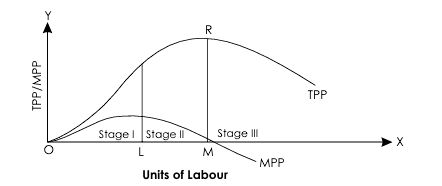
In the diagram, the Total Product (TP) and Marginal Product (MP) curves illustrate the relationship between labor input and output. Key points include:
- Stage I: TP, AP, and MP increase. MP starts to decline at the end of this stage.
- Stage II: TP increases at a diminishing rate. AP declines, and MP decreases until it reaches zero, marking the maximum TP.
- Stage III: TP and AP decline, while MP becomes negative.
Main Points of the Law
- The law of variable proportions is also known as the law of diminishing marginal returns.
- It applies not only to agriculture but also to industries and services.
Reasons for Diminishing Returns
- Variable factors may not be homogeneous.
- Imperfect substitutions among factors.
- Inefficient combinations of inputs.
Importance
This law aids firms in making decisions regarding output levels. Producers typically operate within the second stage, avoiding both the first (increasing returns) and third (negative returns) stages.
Assumptions
- The units of variable factors are homogeneous.
- Some factors can be changed (variable), while others remain constant (fixed).
- Combinations of fixed and variable factors can be adjusted.
- There is no change in the level of technology.
- The law applies only in the short run.
Demand and Supply
Meaning, Demand Function, Law of Demand. Elasticity of Demand, Types, Measurement and importance. Demand Forecasting and its techniques. Concept of Supply, Law of supply.
Cost and Revenue
Concept of Cost, Short run and Lung-run Cost Curves, Relationships among various costs, Break-even Analysis. Revenue, Concept and its Types.