Demand and Supply - HPTU Exam Helper

Meaning of Demand

Demand refers to desire, but in economics, it specifically means a desire that is backed by purchasing power and a willingness to pay the price.

Types of Demand

There are three main types of demand:

Price Demand:
Price demand explains the relationship between the price of a commodity and its demand. There is an inverse relationship; as the price decreases, demand increases, and vice versa. Consequently, the price demand curve slopes downward from left to right.

Dx = f[Px]
Income Demand:
Income demand describes the relationship between consumer income and the demand for goods. Generally, as income rises, consumers purchase more goods; as income falls, they buy less. This indicates a direct proportional relationship, so the income demand curve typically slopes upward from left to right.

Dx = f[y]
- The income demand curve can be divided into two types:
  - Normal (or Superior) Goods: The income demand curve slopes upward, indicating that higher income leads to increased demand for these goods.
  - Inferior Goods: The income demand curve slopes downward, showing that demand decreases as income rises.
Cross Demand:
Cross demand illustrates the relationship between the price of one commodity and the demand for another. The demand for one good is influenced not only by its price but also by the prices of substitute and complementary goods.

Dx = f[Py]
- Substitute Goods: These are goods that can replace each other (e.g., tea and coffee). The cross demand curve for substitutes slopes upward, indicating a direct relationship; as the price of one increases, the demand for the other also increases.
- Complementary Goods: These goods are used together (e.g., milk and sugar for tea). The cross demand curve for complements slopes downward, showing an inverse relationship; as the price of one increases, the demand for the other decreases.

Changes in Demand: Changes in demand can occur due to variations in determinants. These changes can be categorized as:

Extension and Contraction of Demand:
When price changes while other factors remain constant, demand may extend (increase) or contract (decrease). A decrease in price leads to an extension of demand, while an increase in price results in a contraction. This can be illustrated with a single demand curve.
Increase and Decrease of Demand:
When the price is constant but other determinants change, demand may increase or decrease. This results in new demand curves being formed:
- An increase in demand shifts the demand curve to the right.
- A decrease in demand shifts the demand curve to the left.

Demand Function

The demand function represents the relationship between the quantity demanded for a commodity and various determinants. It can be expressed mathematically as:

Dn = f(Pn,Ps,Pc,Y,T)

Where:

Dn = Demand for commodity
f = Functional relationship
Pn= Price of commodity
Ps= Price of substitute goods
Pc= Price of complementary goods
Y = Income of the consumer
T = Taste and preferences of the consumer

Law of Demand in terms of Demand function: The Law of Demand states that, for a given commodity , the quantity demanded (Dn) is inversely related to its price (Pn), assuming all other factors remain constant. These factors include:

Ps: Price of substitute goods
Pc: Price of complementary goods
Y: Consumer income
T: Consumer tastes and preferences

Determinants of demand:

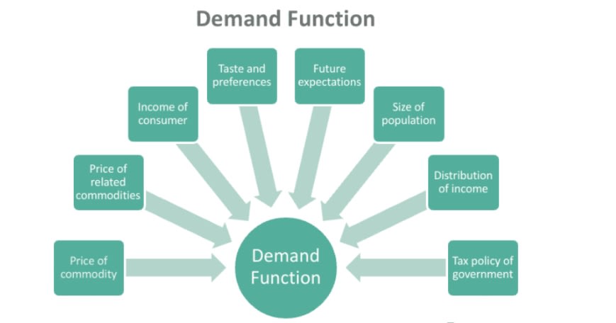
The demand for any commodity is depend upon so many factors. These factors are called determinants of demand. These determinants interact to shape consumer behavior and overall demand for goods, reflecting how market dynamics can change based on various factors.They are:

Price of the goods: The demand for any commodity firstly depends upon its price. When the price rises demand decreases,when the prices falls demand increases.
Prices of the substitute goods: The demand for any commodity not only depends upon its price but also the prices of its substitute goods. For example, tea and coffee. Here the demand for tea depends upon price of the coffee. If the price of coffee falls, the demand for coffee will rise following the law of demand. Since coffee is the substitute for tea, people will reduce the consumption of tea and increase the consumption ofcoffee, as coffee is now relatively cheaper than tea. So, when the price of coffee falls, the demand fortea will also fall. The essence of this example is that demand for a commodity, Dn and the price of itssubstitute, Ps are directly related.
Prices of the complementary goods: The demand for a commodity also depends upon the price of its complementary goods. For example,car and petrol. Here demand for petrol depends upon price of the car.If the price of petrol rises, the demand for petrol will fall, following the law of demand. Since petrolis complementary to the careople will reduce the demand for car along with petrol. So, whenthe price of petrol rises, the demand for car will fall. This analysis indicates that the demand for acommodity, Dn and the price of its complement, Pc are inversely related.
Income of the consumer: The income of the consumer also influences the demand for a commodity. When the income rises people purchase the more quantity of goods. When the income falls they purchase less quantity of goods.
Tastes and preferences of the consumer: The tastes and preference of the consumer can also determine the demand for a commodity. When the tastes are changed, the demand for goods also changed.
Population: When the population is increased, the demand for goods also increases. When the population decreases demand also decreases.
Climate: The climatic conditions also can influence the demand. In hot climatic conditions cold drinks aredemanded. In rainy season umbrellas are demanded.

Law of Demand

The law of demand states that, all else being equal, if the price of a good rises, the quantity demanded decreases, and if the price falls, the quantity demanded increases. This reflects an inverse relationship between price and quantity demanded, expressed as

Dx = f(Px).

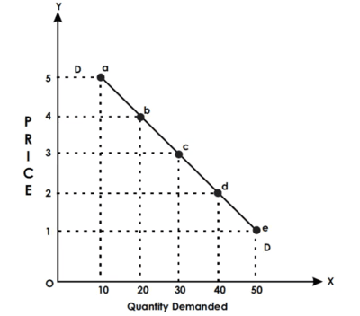
Demand Schedule

A demand schedule displays the quantities of a good demanded at different price levels. There are two main types of demand schedules:

Individual Demand Schedule
Market Demand Schedule

Individual Demand Schedule: This shows the quantity demanded by a single consumer at various prices in market.

Price	Demand
5	10
4	20
3	30
2	40
1	50

Individual Demand Curve

From the demand schedule we can derive demand curve:

Market Demand Schedule

This shows the quantity demanded by a single consumer at various prices in market. A market demand schedule displays the total quantity of a good demanded by all consumers in the market at different price levels. It is derived by summing the individual demand schedules of all consumers.

Price of Good 'x'	Demand
	A	B	C	Demand (A+B+C)
10	100	150	50	500
8	125	200	60	385
6	175	250	80	505
4	250	300	110	660
2	350	400	150	900

Market Demand Curve:

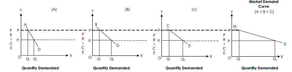
Conclusion: Whether the individual demand curve or market demand curve slopes downwards from left to right because there is an inverse relationship between price and demand.

Causes for falling Nature of Demand Curve, ie.Downward Slope Curve

Law of Diminishing Marginal Utility The law of diminishing marginal utility states that as the quantity of a good consumed increases, the marginal utility derived from each additional unit decreases. Consequently, consumers are more likely to demand greater quantities when prices are lower, which explains why the demand curve slopes downward from left to right.
Substitution Effect When the price of commodity 'X' rises relative to commodity 'Y', consumers will purchase less of 'X' and more of 'Y', which has become relatively cheaper. This behavior is known as the substitution effect, contributing to the downward slope of the demand curve.
Income Effect The income effect indicates that when the price level falls, the real income of consumers effectively increases, allowing them to purchase more goods. This results in higher demand when prices drop.
New Buyers A decrease in the price of a commodity attracts new consumers because the good becomes more affordable. Thus, demand rises as prices fall.
Old Buyers When the price of a good decreases, existing consumers tend to purchase more of that good, leading to an increase in demand. This further illustrates why the demand curve slopes downward.

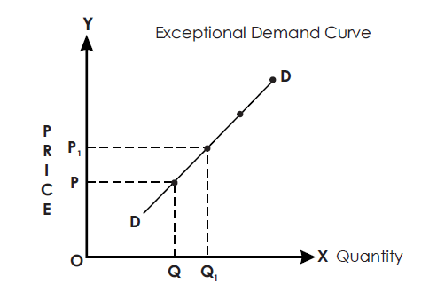
Exceptions to the Law of Demand

While the law of demand generally states that price and quantity demanded are inversely related, there are exceptions where higher prices may lead to increased demand:

Giffen Paradox (Necessary Goods): For certain necessary goods, such as bread, low-income consumers may buy more as prices rise, defying the law of demand. This phenomenon is known as the Giffen Paradox.
Speculation: When consumers anticipate that the price of a commodity will continue to rise, they may buy more at higher prices than they would at lower prices, contrary to the law of demand.
Conspicuous Consumption: Some goods, like luxury cars and diamond jewelry, are purchased to showcase status. Demand for these goods may increase as prices rise, rather than decrease.
Speculative Market: In the stock market, consumers may buy shares as prices rise, expecting further increases. Conversely, they may buy less when prices fall due to expectations of further declines.
Bandwagon Effect: Consumer demand can be influenced by social trends. If a certain trend, like playing golf, becomes fashionable, demand for related goods may increase even if their prices rise.
Illusion: Some consumers may mistakenly believe that higher-priced goods are of better quality. If the price of such goods falls, they may perceive a loss of quality and choose not to buy, which contradicts the law of demand.

Elasticity of Demand

Meaning of Elasticity of Demand: Elasticity refers to the sensitivity or responsiveness of one variable to changes in another variable. Elasticity of demand specifically measures how the quantity demanded of a good responds to changes in its determinants, such as price, consumer income, and the prices of related goods.

Types of Elasticity of Demand: There are three main types of elasticity of demand:

Price Elasticity of Demand
Income Elasticity of Demand
Cross Elasticity of Demand

Price Elasticity of Demand

Definition: “Elasticity of demand measures the degree of responsiveness of demand to changes in price.” – Mrs. John Robinson.

“Elasticity of demand in a market varies based on how much demand increases or decreases in response to a given change in price.” – Alfred Marshall

Price Elasticity of demand illustrates the relationship between the proportionate change in demand and the proportionate change in price. It shows how much a change in price leads to a corresponding change in demand.

The formula for elasticity of demand is:

$E_p = \frac{\text{Proportionate Change in Demand}}{\text{Proportionate Change in Price}}$

$E_p = \frac{\frac{dq}{q}}{\frac{dp}{p}}$

$E_p = \frac{dq}{dp} \times \frac{p}{q}$

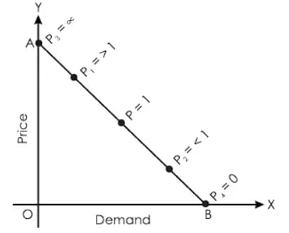
Types of Price Elasticity of Demand: There are five types of price elasticity of demand:

Perfectly Elastic Demand (Ep = ∞)
Perfectly Inelastic Demand (Ep = 0)
Relatively Elastic Demand (Ep > 1)
Relatively Inelastic Demand (Ep < 1)
Unitary Elastic Demand (Ep = 1)

Perfectly Elastic Demand (Ep = ∞): Perfectly elastic demand occurs when a change in demand happens without any change in price. In this case, consumers are willing to purchase any quantity at a specific price, and the demand can increase or decrease infinitely without affecting the price. The value of Ep is infinite. The demand curve in this scenario is parallel to the OX axis, indicating that the quantity demanded remains constant at a given price.
Perfectly Inelastic Demand (EP = 0): When the price changes, if there is no change in the quantity demanded, it is said to exhibit perfectly inelastic demand. This means that regardless of whether the price increases or decreases, the quantity demanded remains constant. In this case, the price elasticity of demand (EP) equals 0. The demand curve for perfectly inelastic demand is vertical, parallel to the Y-axis.
Relatively Elastic Demand (e.g., Luxury Goods): Relatively elastic demand occurs when the proportionate change in quantity demanded is greater than the proportionate change in price. This means that a small change in price leads to a larger change in demand. In this case, the price elasticity of demand (EP) is greater than one. The demand curve for relatively elastic demand slopes downward from left to right.
Relatively Inelastic Demand (e.g., Necessary Goods): Relatively inelastic demand occurs when the proportionate change in quantity demanded is less than the proportionate change in price. This means that a larger change in price leads to a smaller change in demand. In this case, the price elasticity of demand (EP) is less than one. The demand curve for relatively inelastic demand slopes downward from left to right but is steeper than that of relatively elastic demand.
Unitary Elastic Demand: Unitary elastic demand occurs when the proportionate change in quantity demanded is equal to the proportionate change in price. This means that the changes in demand and price are the same. In this case, the price elasticity of demand (EP) is equal to 1. Generally, comfort goods exhibit unitary elastic demand. The demand curve for unitary elastic demand also slopes downward from left to right, but it is shaped like a rectangular hyperbola.

Income Elasticity of Demand

Income elasticity of demand measures the proportionate change in quantity demanded in response to a proportionate change in income. It indicates how much a change in income affects demand. The formula can be expressed as:

$E_p = \frac{\text{Proportionate Change in Demand}}{\text{Proportionate Change in Income}}$

$E_y = \frac{\frac{dq}{q}}{\frac{dy}{y}}$

$E_y = \frac{dq}{dy} \times \frac{y}{q}$

Types of Income Elasticity:

Perfectly Elastic Income Demand (Ey = ∞)
Perfectly Inelastic Income Demand (Ey = 0)
Relatively Elastic Income Demand (Ey > 1)
Relatively Inelastic Income Demand (Ey < 1)
Unitary Elastic Income Demand (Ey = 1)

1. Perfectly Elastic Income Demand: Perfectly elastic income demand occurs when demand changes while income remains constant. This means that demand can increase or decrease without any change in income. In this case, the value of EY is infinite, and the demand curve is horizontal (parallel to the X-axis).

2. Perfectly Inelastic Income Demand: Perfectly inelastic income demand occurs when income changes but demand remains constant. This means that demand does not change, regardless of whether income increases or decreases. Here, the value of EY is zero, and the demand curve is vertical (parallel to the Y-axis).

3. Relatively Elastic Income Demand: Relatively elastic income demand occurs when the proportionate change in demand is greater than the proportionate change in income. This means that a small change in income leads to a larger change in demand. Here, the value of EY is greater than one, and the demand curve slopes downward from left to right.

4. Relatively Inelastic Income Demand: Relatively inelastic income demand occurs when the proportionate change in demand is less than the proportionate change in income. This means that a larger change in income results in a smaller change in demand. Here, the value of EY is less than one, and the demand curve slopes upward from left to right.

5. Unitary Elastic Income Demand: Unitary elastic income demand occurs when the proportionate change in demand is equal to the proportionate change in income. This means that changes in income result in proportional changes in demand. Here, the value of EY is one, and the demand curve slopes upward from left to right.

Cross Elasticity of Demand: Cross elasticity of demand measures the proportionate change in the quantity demanded of one commodity in response to a proportionate change in the price of another commodity. It indicates how much a change in the price of one good affects the demand for another good

$E_p = \frac{\text{Proportionate Change in Demand for goods 'x'}}{\text{Proportionate Change in Price for goods 'y'}}$

$E_c = \frac{\frac{dq_x}{q_x}}{\frac{dp_y}{p_y}}$

$E_c = \frac{dq_x}{dp_y} \times \frac{p_y}{q_x}$

Measurements of Elasticity of Demand

There four methods to measure the elasticity of demand:

Percentage method
Total outlay method
Point method
Arc method

Percentage Method: This method calculates elasticity by finding the percentage change in demand and the percentage change in price. The formula used is:

$E_p = \frac{\text{Proportionate Change in Demand}}{\text{Proportionate Change in Price}}$
Total outlay Method:

In this method, the relationship between price and total expenditure is used to determine elasticity.
- Relatively Elastic Demand (EP > 1): If total expenditure increases when the price falls and decreases when the price rises, the demand is said to be relatively elastic.
- Unitary Elastic Demand (EP = 1): If total expenditure remains constant regardless of whether the price increases or decreases, the demand is classified as unitary elastic.
- Relatively Inelastic Demand (EP < 1): If total expenditure decreases when the price falls and increases when the price rises, the demand is considered relatively inelastic.
  
  Price Demand Total Outlay
  9 40 360
  8 50 400
  7 60 420
  6 70 420
  5 80 400
  4 90 360
Point Method:

In the point method, the elasticity of demand is measured at a specific point on the demand curve. The following formula is used:

$E_p = \frac{\text{Lower Segment}}{\text{Upper Segment}}$

Let us assume the total length of the demand curve is 40 cm, with segment AB representing the demand curve. The elasticity of demand can be calculated at various points along this curve using the above formula.

$E_p \text{ at point } 'P' = \frac{PB}{PA} = \frac{20}{20} = 1$

$E_p \text{ at point } 'P_1' = \frac{p_1 B}{p_1 A} = \frac{10}{30} = 0.33$

$E_p \text{ at point } 'P_2' = \frac{p_2 B}{p_2 A} = \frac{30}{10} = 3$

$E_p \text{ at point } 'P_3' = \frac{p_3 B}{p_3 A} = \frac{40}{0} = \infty$

$E_p \text{ at point } 'P_4' = \frac{p_4 B}{p_4 A} = \frac{0}{40} = 0$
Arc Method: When there are small changes in demand and price, it may not be possible to measure elasticity using the point method. Therefore, the arc method is introduced. In this method, the following formula is used:

Price Demand
$2P_1$ $1000 \, q_1$
$1P_2$ $2000 \, q_2$

$E_p = \frac{\text{change in demand}}{\text{1st demand + 2nd demand}} + \frac{\text{change in price}}{\text{1st demand + 2nd demand}}$

$\frac{q_2 - q_1}{q_1 + q_2} + \frac{p_2 - p_1}{p_1 + p_2}$

$\frac{1000}{1000 + 2000} + \frac{-1}{112}$

$\frac{1000}{3000} + \frac{3}{-1} = -1$

= unitary

Price	Demand	Total Outlay
9	40	360
8	50	400
7	60	420
6	70	420
5	80	400
4	90	360

Price	Demand
$2P_1$	$1000 \, q_1$
$1P_2$	$2000 \, q_2$

This formula allows for the calculation of elasticity over a range of prices and quantities, rather than at a single point.

Importance of Elasticity of Demand

The concept of elasticity of demand is crucial in both government finance and trade.

If a product has elastic demand, businesses tend to set lower prices; if demand is inelastic, they may set higher prices.

Business Decision: If a product has elastic demand, businesses tend to set lower prices; if demand is inelastic, they may set higher prices.
Monopolist Pricing: A monopolist will charge higher prices in markets where demand is inelastic and lower prices where demand is elastic for the same good.
Determination of Factor Prices: Elasticity of demand helps determine the prices of production factors. Inelastic demand for a factor results in higher prices, while elastic demand leads to lower prices.
International Trade: If the demand for a country's exports is inelastic, it benefits from favorable terms of trade. Conversely, if export demand is more elastic than import demand, the country may face unfavorable terms.
Government Policy: Elasticity informs government decisions on which industries should be designated as public utilities for state operation.

Determinants of Elasticity of Demand

Nature of the Commodity: Demand for necessities (e.g., rice, salt) is generally inelastic, while demand for luxuries (e.g., TVs, diamonds) is more elastic. Comfort goods typically have unitary elastic demand.
Availability of Substitutes: The presence of substitute goods makes demand more elastic. For example, various soap brands (e.g., Lux, Pears) can be easily substituted.
Variety of Uses: Goods with multiple uses (e.g., milk, coal) tend to have more elastic demand.
Possibility of Postponement of Consumption: Goods that can be postponed for purchase (e.g., luxury items) usually have elastic demand. In contrast, life-saving medicines have inelastic demand due to the urgency of their need.
Durability of Goods: Durable goods generally have less elastic demand, while perishable goods tend to have more elastic demand.

Demand Forecasting and Techniques

The success of a business firm heavily relies on effective demand forecasting, which is the estimation of future demand for a product. Demand forecasting is crucial for guiding production, resource allocation, pricing strategies, and inventory management. By accurately forecasting demand, firms can minimize costs associated with overproduction or stockouts, ensure timely fulfillment of customer needs, and optimize their supply chains.

Methods of Demand Forecasting:

Expert Opinion Method
Survey of Buyers' Intentions
Collective Opinion Method
Controlled Experiments
Statistical Method

Importance of Demand Forecasting

Demand forecasting holds a significant place in strategic business planning. For companies, an accurate demand forecast helps improve customer satisfaction by aligning production schedules with demand, thereby avoiding stockouts or delays. Furthermore, it aids in budgeting and financial planning, as companies can allocate resources more effectively when they anticipate future demand. In a broader economic context, accurate demand forecasting contributes to efficient market operations and stability by reducing the risks associated with supply-demand mismatches.

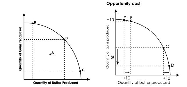
Production Possibility Curve (PPC)

The Production Possibility Curve (PPC), also known as the production possibility frontier or transformation curve, illustrates the various combinations of two commodities that an economy can produce with its given resources and technology.

Main Points:

Downward Slope: The PPC slopes downward from left to right because increasing the production of one commodity results in the foregone production of another.
Concave Shape: The curve is concave to the origin, indicating that the marginal rate of transformation (MRT) increases as production shifts from one good to another.
Marginal Rate of Transformation (MRT): The slope at any point on the PPC represents the MRT, which indicates the rate at which production of one good can be redirected to produce another, also referred to as opportunity cost.
Example: At point D on the PPC, moving right to produce more butter means sacrificing the production of guns. As production shifts, specialized inputs for gun production become less useful for butter production, leading to a concave curve because the MRT decreases.

Key Notes:

A straight-line PPC indicates constant opportunity cost.
Points on the PPC represent efficient combinations of resources.
Points beyond the PPC are unattainable combinations.
Shifts of the PPC signify economic growth.
Points below the PPC indicate underutilized resources or unemployment.

Importance of PPC in Economic Planning

The PPC serves as a crucial analytical tool for economic planning. It visually represents the trade-offs and opportunity costs associated with resource allocation, aiding policymakers in understanding the consequences of choosing one allocation strategy over another. Additionally, it helps in assessing the productive efficiency of an economy, guiding decisions on how to utilize resources optimally. The PPC is also fundamental in illustrating economic growth: shifts in the PPC reflect increases in an economy's capacity to produce goods and services due to technological advancements or improvements in resource availability.

Solving Economic Problems with the PPC

What to Produce: Choosing a point on the PPC helps address the economic question of "what to produce," ensuring full and efficient resource utilization. The “invisible hand,” or price system, guides this process. If a product is underproduced, demand will exceed supply, driving up prices and prompting producers to increase output.
How to Produce: Once the first question is addressed, the next is "how to produce." The choice between labor-intensive and capital-intensive techniques depends on the relative costs of labor and capital.
For Whom to Produce: The question of "for whom to produce" is determined by purchasing power, which is influenced by the price of labor (wage rates) and overall income levels. Thus, the price system helps allocate commodities to consumers effectively.

Concept of Supply

Meaning of Supply: There is a difference between the stock of goods and the supply of goods. Supply refers to the quantity of a product that a seller is willing and able to sell at a particular price, in a specific market, during a specified period of time.

Determinants of Supply: The supply of any commodity depends on several factors, known as the determinants of supply. These include:

Price of the Goods
The price of goods is a primary determinant of supply. Producers tend to supply more goods when prices are high and supply fewer goods when prices are low.
Goals of the Firm
Firms may pursue various goals, such as profit maximization, sales maximization, or employment maximization. If a firm aims to maximize profit, a higher profit from the sale of a commodity will lead to a greater quantity supplied, and vice versa.
Input Prices
Producers are more likely to supply more when input prices are low, as this reduces production costs. Conversely, when input prices rise, supply tends to decrease.
Technology New technology typically helps to save inputs and reduces the costs and time required to produce output. Improved technology can enhance the supply of goods.
Government Policies
Government policies regarding taxes and subsidies significantly affect supply. Higher taxes on goods can discourage production, leading to a decrease in supply, while subsidies can encourage producers to supply more.
Expectations about Future Prices If producers expect an increase in the price of a commodity, they may supply less at the current price and hold back stock to sell at a higher price later. Conversely, if they anticipate a fall in future prices, they may increase current supply to sell before prices drop (as seen with fruit sellers).
Prices of Other Commodities An increase in the prices of other commodities may make the production of those goods more attractive. Consequently, if the price of one commodity remains unchanged while the prices of others rise, the supply of the original commodity may decrease.
Number of Firms in the Market Market supply is the sum of the supplies from individual firms. Therefore, a decrease in the number of firms in the market reduces overall supply.
Natural Factors Supply can be affected by natural conditions, such as weather. Events like droughts, floods, extreme weather, and pest infestations can disrupt crop production and the supply of raw materials, impacting overall supply.

Law of Supply

The law of supply explains the functional relationship between the price of a good and the quantity supplied. When all other factors remain constant, if the price rises, the supply also increases; conversely, if the price falls, the supply decreases. This indicates a direct proportional relationship between price and supply.

Supply Schedule

A supply schedule shows the various quantities of a good that are supplied at different price levels.

Types of Supply Schedules:

Individual Supply Schedule:
This schedule displays the quantities of a good supplied by an individual seller or producer at various price levels.

Price of X Supply of X Goods
500 0
1000 10
1500 30
2000 55
2500 90

Supply Curve: From the above supply schedule, a supply curve can be drawn, showing the upward slope of supply as price increases.
Market Supply Schedule:
This schedule reflects the total quantities of a good supplied by all producers or sellers at various price levels. The total supply or market supply is obtained by summing the supplies of all sellers. Both the individual and market supply curves slope upward from left to right, illustrating the direct relationship between price and supply.

Price of X	Supply of X Goods
500	0
1000	10
1500	30
2000	55
2500	90

Exceptions to the Law of Supply

Land or Agricultural Goods:
The supply curve for agricultural goods is often vertical (parallel to the OY-axis) since the supply cannot easily change with price.
Rare Goods:
For rare goods, the supply remains fixed regardless of price changes, resulting in a vertical supply curve.
Supply of Labor:
The supply curve for labor can be backward-bending. Initially, as wage levels increase, labor supply increases, but beyond a certain wage level, workers may prefer more leisure time, leading to a decrease in labor supply.

Change in Supply

Changes in the determinants of supply can lead to shifts in supply. These changes can be categorized as:

Extension and Contraction of Supply:
When the price changes, the supply may extend or contract. An increase in price results in an extension of supply, while a decrease in price leads to a contraction of supply. This can be illustrated with a single supply curve.
Increase and Decrease of Supply:
When supply changes due to alterations in determinants while the price remains constant, new supply curves are formed.
- An increase in supply shifts the supply curve to the right.
- A decrease in supply shifts the supply curve to the left.

Supply Function

The supply function describes the relationship between supply and the factors that determine it. This relationship can be expressed with the equation:

$S_x = f(P_x, P_I, T, W, G_P)$

Where:

$S_x$ = Supply of good
$f$ = Functional relationship
$P_x$ = Price of good
$P_I$ = Price of inputs (factors)
$T$ = Technology
$W$ = Weather conditions
$GP$ = Government policy

How's article quality?

Page Contents