Concept of Cost
Cost of Production
Cost refers to the expenditure incurred by a producer or firm to produce goods and services, represented as C=f(Q), where (Q) is the quantity produced.
Types of Cost:
-
Money Cost: This is the cost incurred when remuneration for the factors of production is paid in the form of money. Examples include rent paid for land and wages paid to laborers.
-
Real Cost: Introduced by Alfred Marshall, real cost encompasses the exertions and sacrifices involved in the production process. This includes all forms of labor and the efforts required to save capital. In essence, it refers to the true sacrifices made in producing a good.
-
Economic Costs: Economic costs are the total expenses incurred by a firm in producing a commodity, which include:
- Explicit Costs: Actual payments made by a firm for purchasing or hiring resources, such as rent for land, wages for labor, expenditure on raw materials, and interest on borrowed money. These costs are recorded in the firm's accounting books.
- Implicit Costs: Implicit costs associated with the factors of production owned by the producer, which are not directly recorded in the accounts. Examples include the rental value of owned land and the foregone interest on the entrepreneur's own capital.
- Normal Profit: The minimum profit required to keep an entrepreneur in the production process.
Thus, the formula for economic cost can be summarized as:
Economic Cost = Explicit Cost + Implicit Cost + Normal Profit
-
Opportunity Cost: Opportunity cost refers to the value of the next best alternative that is forgone when a choice is made. Given the scarcity of resources, choosing one commodity means forgoing another. For instance, if land can be used to grow either wheat or rice, the opportunity cost of choosing to grow rice is the potential yield of wheat that is sacrificed.

Suppose a farmer has a piece of land that can produce either 50 quintals (ON) of rice or 40 quintals (OM) of wheat. If the farmer chooses to produce 50 quintals of rice (ON), he cannot produce any wheat. Therefore, the opportunity cost of producing 50 quintals of rice is 40 quintals of wheat.
The farmer can also produce any combination of the two crops along the production possibility curve (PPC) MN. Let’s assume that the farmer is operating at point A on the production possibility curve, where he produces an amount of rice represented by OD and an amount of wheat represented by OC.
If the farmer decides to move to point B on the production possibility curve, he must reduce his production of wheat from OC to OE in order to increase his production of rice from OD to OF. This means that the opportunity cost of increasing rice production by DF amount is the corresponding decrease in wheat production by CE amount.
Cost Function The cost function describes the relationship between the cost of production and the physical quantity of output, represented as:
Short-Run Costs:
In the short run, the cost of production can be divided into two types:
-
Fixed Costs:
Fixed costs do not change with variations in output. This means that regardless of whether output increases or decreases, these costs remain constant. Even when production is zero, fixed costs are still incurred. The total fixed cost (TFC) curve is parallel to the x-axis.
Examples: Expenditures on land, buildings, salaries of permanent employees, interest payments, and insurance premiums.
-
Variable Costs:
Variable costs change with the level of output. When output increases, these costs increase, and when output decreases, they decrease as well. If production is stopped, variable costs become zero. The total variable cost (TVC) curve slopes upward from left to right and starts from the origin.
Examples: Expenditures on raw materials, power, fuel, and wages for daily laborers.
| Aspect | Fixed Costs | Variable Costs |
|---|---|---|
| Definition | Costs that remain constant regardless of output levels. | Costs that change with the level of output. |
| Behavior with Output | Do not vary with changes in output. | Increase as output rises and decrease when output falls. |
| Incurred at Zero Output | Incurred even when production is zero. | Become zero if production stops. |
| Examples | Rent for land, building expenses, salaries of permanent staff, interest payments, insurance premiums. | Expenditures on raw materials, power, fuel, wages for hourly workers. |
| Characteristics | Associated with fixed factors of production; remain constant even if production ceases. | Linked to variable factors of production; can fluctuate based on output. |
Total Costs:
Total costs (TC) are calculated by adding fixed and variable costs:
As output increases, total costs also rise, and they fall when output decreases. The total cost curve slopes upward, reflecting a direct relationship between output and total cost, starting above the origin at the level of total fixed costs.
Short Run Cost Curve
The total cost (TC) relationship with total fixed cost (TFC) and total variable cost (TVC) at various levels of output. Including the output levels, TFC, TVC, and TC values in a table format.
Short Run Cost: In the short run, at least one input is fixed, while the quantities of other inputs can be varied. Typically, factors such as land and machinery remain constant during this period. In contrast, inputs like labor and capital can be adjusted over time. In the short run, expansion occurs primarily by hiring more labor and utilizing existing capital more efficiently. The size of the plant or building cannot be increased in the short run.
Cost Table
| Output | TFC | TVC | TC |
|---|---|---|---|
| 0 | 20 | 0 | 20 |
| 1 | 20 | 8 | 28 |
| 2 | 20 | 14 | 32 |
| 3 | 20 | 18 | 38 |
| 4 | 20 | 22 | 42 |
| 5 | 20 | 28 | 48 |
| 6 | 20 | 32 | 52 |
| 7 | 20 | 40 | 60 |
| 8 | 20 | 45 | 65 |
Explanation:
- TFC (Total Fixed Cost): Remains constant at 20 across all levels of output.
- TVC (Total Variable Cost): Increases as output increases, reflecting the costs associated with producing additional units.
- TC (Total Cost): Calculated as . This value increases as output rises, showing the cumulative costs of production.
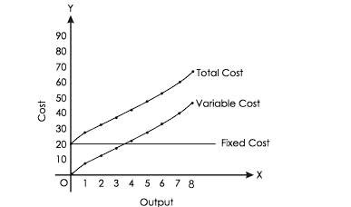
Graph Explanation
- The TFC curve would be a horizontal line at 20, indicating that fixed costs do not change with output.
- The TVC curve would slope upward, starting from the origin (0,0) and increasing with output.
- The TC curve would start at 20 and slope upwards, showing the total costs at each output level.
Other Cost Curves in the Short Run
From the data provided, we can derive various cost concepts. Below is a table summarizing the costs for different output levels.
| Output | TFC | TVC | TC | AFC | AVC | AC | MC = TCn - TCn-1 |
|---|---|---|---|---|---|---|---|
| 0 | 20 | 0 | 20 | - | - | - | - |
| 1 | 20 | 8 | 28 | 20 | 8 | 28 | 8 |
| 2 | 2- | 14 | 52 | 10 | 7 | 16 | 6 |
| 3 | 20 | 18 | 38 | 6.66 | 6 | 19 | 6 |
| 4 | 20 | 22 | 42 | 5 | 5.5 | 21 | 4 |
| 5 | 20 | 28 | 48 | 4 | 5.6 | 24 | 4 |
| 6 | 20 | 32 | 52 | 3.33 | 5.33 | 26 | 4 |
| 7 | 20 | 40 | 60 | 2.85 | 5.71 | 30 | 8 |
| 8 | 20 | 45 | 65 | 2.5 | 5.63 | 32.5 | 5 |
Definitions of Costs:
-
Average Fixed Cost (AFC):
-
Definition: The average total fixed cost per unit of output, calculated as:
-
Curve Shape: Slopes downward from left to right, represented as a rectangular hyperbola.

-
-
Average Variable Cost (AVC):
-
Definition: The average total variable cost per unit of output, calculated as:
-
Curve Shape: U-shaped, indicating that costs decrease initially with increased output, then increase as diminishing returns set in.

-
-
Average Cost (AC):
-
Definition: The average total cost per unit of output, calculated as:
-
Curve Shape: Also U-shaped, reflecting the combined behavior of AFC and AVC.

-
-
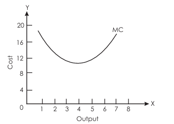
Marginal Cost (MC):
-
Definition: The additional cost incurred from producing one more unit of output. It is calculated as the change in total cost:
-
Curve Shape: U-shaped, similar to AVC and AC, indicating that initial production efficiency is followed by increasing costs as output rises.
-
Graphical Representation:
- AFC Curve: Decreases as output increases.
- AVC Curve: U-shaped, initially decreasing and then increasing.
- AC Curve: U-shaped, starting higher and reflecting the influence of both fixed and variable costs.
- MC Curve: U-shaped, indicating the cost of producing additional units.
Difference Between Marginal Cost and Average Cost
Average Cost (AC):
-
Average cost refers to the average total cost per unit of output. It is calculated by dividing total cost TC by the number of units produced (Q):
-
Average cost can also be expressed as the sum of average fixed cost (AFC) and average variable cost (AVC):
Marginal Cost (MC):
-
Marginal cost is the additional cost incurred to produce one more unit of output. It is calculated as the change in total cost resulting from the production of an additional unit:
Long-Run Cost Curve
In the short run, a firm operates with a fixed scale of plant, which corresponds to a specific short-run average cost (SRAC) curve. This means that the firm can only operate at a particular scale of production. However, in the long run, a firm can choose among various sizes of plants and can transition from one scale of production to another.
This relationship can be illustrated in the following diagram:
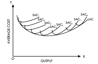
In the diagram, multiple short-run average cost curves (SRAC) represent different plant sizes. The long-run average cost (LAC) curve is tangent to each of the short-run average cost curves. This tangency indicates the least average cost achievable for producing a given quantity of output when the scale of the plant is varied.
Main Points:
- The LAC curve is U-shaped and is often referred to as the planning curve or envelope curve.
- Similarly, the long-run marginal cost (LMC) curve is also U-shaped.
Relation Among Various Costs
-
MC and AC Relationship
The marginal cost curve is typically U-shaped, reflecting changes in production efficiency.
In the following diagram, we can illustrate the relationship between MC and AC:

In the first stage of production:
- Both MC and AC are decreasing.
- The MC is less than the AC, which means the MC curve lies below the AC curve.
In the second stage of production:
- Both MC and AC are increasing.
- The MC becomes greater than the AC, so the MC curve lies above the AC curve.
The point at which the MC curve intersects the AC curve corresponds to the minimum average cost. This is often referred to as the point of "normal profit," where the firm is neither making abnormal profits nor losses.
- When MC is less than AC, AC is decreasing. When MC is greater than AC, AC is increasing. The MC curve intersects the AC curve at its minimum point.
-
Relationship Between AVC and MC
The relationship between AVC and MC curves is similar to that of Average Cost (AC) and MC.
-
Derived from Total Variable Cost:
- Both AVC and MC are derived from Total Variable Cost (TVC). AVC represents the TVC per unit of output, while MC is the additional cost incurred when producing one more unit of output.
-
U-Shaped Curves:
- Both AVC and MC curves are U-shaped due to the Law of Variable Proportions.
The relationship between AVC and MC can be better illustrated with the following schedule and diagram.
Table
Output (units) TVC (Rs.) AVC (Rs.) MC (Rs.) Phase 0 0 - - - 1 6 6 6 I (MC < AVC) 2 10 5 4 3 15 5 5 II (MC = AVC) 4 24 6 7 III (MC > AVC) 5 35 7 9 6 45 8 11 
Key Points:
-
When MC is less than AVC, AVC decreases as output increases, which occurs until the second unit of output.
-
When MC equals AVC (at the third unit of output), AVC remains constant and reaches its minimum point (point B).
-
When MC is greater than AVC, AVC begins to rise with an increase in output, starting from the fourth unit of output.
-
Thereafter, both AVC and MC rise, but MC increases at a faster rate than AVC. As a result, the MC curve is steeper compared to the AVC curve.
-
-
Relationship Between TVC and MC
Marginal Cost (MC) represents the additional cost incurred when one more unit of output is produced. Therefore, Total Variable Cost (TVC) can be understood as the summation of the MCs for all units produced. If we assume output is perfectly divisible, then the total area under the MC curve will equal the TVC.

In the diagram, at the output level OQ, TVC is represented by the shaded area OPLQ. This area visually illustrates the total variable cost associated with producing OQ units of output.
-
Relationship between TC and MC
The main points of relationship between TC and MC are:
-
Marginal cost is the addition to total cost, when one more unit of output is produced. MC is calculated as:
-
When TC rises at a diminishing rate, MC declines.
-
When the rate of increase in TC stops diminishing, MC is at its minimum point, i.e. point E
-
When the rate of increase in total cost starts rising, the marginal cost is increasing.

-
-
Relationship Between AC, AVC, and MC
The relationship between AC, AVC, and MC can be illustrated with the following schedule and diagram.
Table : Relationship between AC, AVC, and MC
Output (units) TVC (Rs.) AC (Rs.) AVC (Rs.) MC (Rs.) 0 0 — — — 1 6 18 6 6 2 10 11 5 4 3 15 9 5 5 4 24 9 6 9 5 35 9.40 7 11 
Key Points:
-
When MC is Less Than AC and AVC:
- When MC is less than both AC and AVC, both curves fall as output increases.
-
When MC Equals AC and AVC:
- When MC becomes equal to AC and AVC, both become constant. The MC curve intersects the AC curve at point ‘A’ and the AVC curve at point ‘B’, which represent their minimum points.
-
When MC is Greater Than AC and AVC:
- When MC is greater than both AC and AVC, both curves rise as output increases.
-
Break-Even Analysis
Break-even analysis is an essential economic tool that determines the point beyond which a company earns a profit. It helps businesses calculate the volume of products that must be sold to cover all initial costs of investment. Reaching this break-even point means that a company is no longer in a state of loss.
What is the Break-Even Point?
In a business context, the break-even point (BEP) is the level at which total expenses equal total revenue. This indicates that a business has covered all its expenses and is no longer operating at a loss.
Accurately calculating the break-even point is vital for business planning and financial management.
Break-Even Point Formula
The break-even point can be calculated using the following formula:
=
Where:
- Fixed Cost: Costs incurred by a business that do not vary with the volume of production (e.g., rent, loans, insurance premiums).
- Variable Cost: The cost incurred to produce one unit of a product.
Example of Break-Even Analysis
Case Study: ABC Enterprises
| Parameter | Value |
|---|---|
| Total Fixed Costs | Rs. 50,000 |
| Variable Cost per Unit | Rs. 30 |
| Selling Price per Unit | Rs. 50 |
Calculation:
From the above analysis, the break-even point for ABC Enterprises is 2,500 units. This means the company needs to sell at least 2,500 units of the product to cover its fixed and variable costs.
Total Sales at Break-Even Point
To determine the total sales at the break-even point, multiply the break-even quantity by the selling price per unit:
Total Sales = Break-even Point x Selling Price per Unit =
Diagram
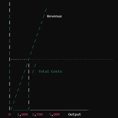
In this diagram:
- The point where the revenue line intersects the total costs line represents the break-even point (2,500 units).
- To the left of this point, the company incurs losses; to the right, it earns profits.
Significance of Break-Even Analysis
-
Determines Volume of Products to be Sold
- Break-even analysis helps companies ascertain the minimum number of units that must be sold to cover total fixed and variable costs. This provides a clear target for sales needed to avoid losses.
-
Deciding Budgets and Targets
- By understanding the operational dynamics through break-even analysis, businesses can effectively plan budgets for various operations. It also enables the setting of achievable production targets.
-
Cost Control
- Fixed and variable costs directly impact profit margins. Break-even analysis allows organizations to assess changes in costs and implement necessary cost-control measures to ensure profitability.
-
Designing Pricing Strategy
- Pricing significantly influences break-even calculations. For instance, increasing the selling price reduces the number of units needed to break even. This insight helps in crafting effective pricing strategies.
-
Margin of Safety Management
- In times of financial uncertainty, break-even analysis aids in managing the margin of safety. It helps determine the minimum sales volume required to avoid losses during downturns.
Margin of Safety Formula:
or
Components of Break-Even Analysis
-
Fixed Costs
- Fixed costs remain constant regardless of the level of production. These include salaries, rent, insurance premiums, and other overhead expenses.
-
Variable Costs
- Variable costs fluctuate based on production levels. These include costs for raw materials, packaging, labor, and other expenses directly tied to production volume.
Break-Even Analysis Formula:
Applications of Break-Even Analysis
-
Planning in New Businesses
- For new ventures, break-even analysis is crucial to evaluate the viability of business plans regarding cost and pricing strategies.
-
Introduction of New Products
- Before launching new products, companies can utilize break-even analysis to determine the feasibility and cost implications, guiding production decisions.
-
Business Model Modification
- Changes in business models (e.g., shifting from retail to wholesale) may necessitate a reevaluation of pricing strategies. Break-even analysis helps assess the need for adjustments.
Concepts of Revenue and its Types
Revenue refers to the income generated by a firm or producer through the sale of goods and services in the market.
There are three key concepts of revenue:
-
Total Revenue (TR): Total revenue is the overall income received by a firm or producer from selling all goods and services in the market. It is calculated by multiplying the price per unit by the total quantity sold. Additionally, total revenue can be understood as the sum of all marginal revenues for each unit sold.
Or
-
Average Revenue (AR): Average revenue is defined as the revenue earned per unit of output sold in the market. It is calculated by dividing total revenue by the number of units sold.
-
Marginal Revenue (MR): Marginal revenue is defined as the additional revenue that a firm or producer earns from selling one more unit of a good or service. It can be calculated as the change in total revenue resulting from the sale of an additional unit.
or
Revenue Curves under Different Markets:
Revenue curves vary across different market structures. In a perfectly competitive market, the average revenue (AR) and marginal revenue (MR) behave differently compared to imperfectly competitive markets.
AR and MR Curves in Perfect Competition
In a perfectly competitive market, the price remains constant because the goods offered are homogeneous. This leads to specific characteristics for the AR and MR curves as output increases. The following table illustrates this relationship:
| Output | Price | Total Revenue (TR) | Average Revenue (AR) | Marginal Revenue (MR) |
|---|---|---|---|---|
| 1 | 10 | 10 | 10 | 10 |
| 2 | 10 | 20 | 10 | 10 |
| 3 | 10 | 30 | 10 | 10 |
| 4 | 10 | 40 | 10 | 10 |
| 5 | 10 | 50 | 10 | 10 |
In this scenario:
- Average Revenue (AR): The average revenue per unit sold remains constant at the market price (Rs. 10).
- Marginal Revenue (MR): The marginal revenue, which is the additional revenue from selling one more unit, also remains constant at Rs. 10.
This indicates that in a perfectly competitive market, the AR and MR curves are horizontal lines at the market price level.
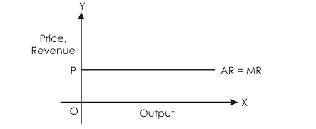
Here AR = MR curve is parallel to ox-axis. Because the price is constant in this market.
MR and AR Curves under Imperfect Market
In an imperfect market, the price changes as the seller adjusts their sales strategy. To increase sales, the seller must reduce the price. As the price decreases, both the average revenue (AR) and marginal revenue (MR) also decline. This relationship can be illustrated in the following schedule:
| Output | Price | Total Revenue (TR) | Average Revenue (AR) | Marginal Revenue (MR) |
|---|---|---|---|---|
| 1 | 10 | 10 | 10 | 10 |
| 2 | 9 | 18 | 9 | 8 |
| 3 | 8 | 24 | 8 | 6 |
| 4 | 7 | 28 | 7 | 4 |
| 5 | 6 | 30 | 6 | 2 |
In this scenario:
- As output increases, the price decreases.
- Average Revenue (AR): The average revenue per unit sold decreases as output increases.
- Marginal Revenue (MR): The marginal revenue also declines with increased output.
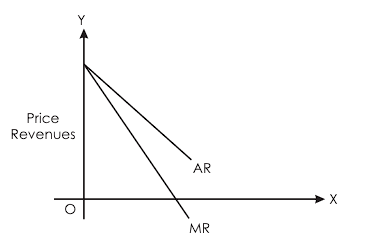
In an imperfect market, both the MR and AR curves slope downwards from left to right. In this case, the MR curve lies below the AR curve.
Additionally, the price is always equal to the average revenue (P = AR) in all markets.