Wave Function

Waves, in general, are associated with quantities that vary periodically. In the case of matter waves, the quantity that varies periodically is called the wave function.

The wave function, represented by $\psi$, associated with matter waves has no direct physical significance as an observable quantity. However, the value of the wave function is related to the probability of finding the particle at a given place at a given time.

The square of the absolute magnitude of the wave function of a particle, evaluated at a particular time and place, is proportional to the probability of finding the particle at that place at that instant.

The wave functions are usually complex. The probability density in such a case is given by $\psi^*$ $\psi$, i.e., the product of the wave function with its complex conjugate, $\psi^*$ being the complex conjugate. Since the probability of finding a particle somewhere is finite, we have the total probability over all space equal to unity. That is

$$\int_{a}^{b} \psi^* \psi \, dV = 1$$

where $dV = dx \: dy\: dz$

This equation is called the normalization condition, and a wave function that obeys this equation is said to be normalized. Further, $\psi$ must be single-valued since the probability can have only one value at a particular place and time. Besides being normalizable, a further condition that $\psi$ must obey is that it and its partial derivatives, $\frac{\partial \psi}{\partial x}$, $\frac{\partial \psi}{\partial y}$ and $\frac{\partial \psi}{\partial z}$ be continuous everywhere.

The important characteristics of the wave function are as follows:

1. $\psi$ must be finite, continuous and single-valued everywhere.
2. $\frac{\partial \psi}{\partial x}$, $\frac{\partial \psi}{\partial y}$ and $\frac{\partial \psi}{\partial z}$ must be finite, continuous and single valued.
3. $\psi$ must be normalisable.

Postulates of Quantum Mechanics

1. State Postulate

   A physical system is completely described by its wave function (state function) $\psi$. The wave function is a complex-valued function of the coordinates of the particles and time.

   • $\psi(x, t)$ contains all the information about the system.
   • The probability density function is given by $|\psi(x, t)|^2$.

2. Observable Postulate

   Every observable in quantum mechanics is represented by a corresponding operator. These operators are Hermitian to ensure real eigenvalues, which correspond to measurable quantities.

   • For example, the position observable is represented by the operator $\hat{x}$, and the momentum observable by $\hat{p} = -i\hbar \frac{\partial}{\partial x}$.

3. Measurement Postulate

   The only possible result of a measurement of an observable is one of the eigenvalues of the corresponding operator.

   • When a measurement is made, the system collapses to an eigenstate of the observable, and the measurement outcome is the eigenvalue associated with that eigenstate.

4. Expectation Value Postulate

   The expectation value (average measurement) of an observable $\hat{A}$ in a state $\psi$ is given by:

   $$\langle A \rangle = \int \psi^*(x) \hat{A} \psi(x) \, dx$$

5. Time Evolution Postulate

   The time evolution of the wave function $\psi(x, t)$ is governed by the Schrödinger equation:

   $$i\hbar \frac{\partial \psi(x, t)}{\partial t} = \hat{H} \psi(x, t)$$

   where $\hat{H}$ is the Hamiltonian operator, representing the total energy of the system.

Schrödinger Equation

The Schrödinger Equation is a mathematical expression that describes the change of a physical quantity over time in scenarios where quantum effects, such as wave-particle duality, are significant. There are two forms of the Schrödinger Equation: the time-dependent Schrödinger Equation and the time-independent Schrödinger Equation.

Derivation of Schrodinger Equation for Time Independent

Consider a system of stationary waves associated with a moving particle. The waves are said to be stationary with respect to the particle. If the position coordinates of the particle are $(x, y, z)$ and $\psi$ is the periodic displacement for the matter waves at any instant of time $t$, then we can represent the motion of the wave by a differential equation as follows:

$$\frac{\partial^2 \psi}{\partial x^2} + \frac{\partial^2 \psi}{\partial y^2} + \frac{\partial^2 \psi}{\partial z^2} = \frac{1}{u^2} \frac{\partial^2 \psi}{\partial t^2} \quad \text{(i)}$$

where $u$ is the velocity of wave associated with the particle. The solution of Eq. (i) gives $\psi$ as a periodic displacement in terms of time, i.e.,

$$\psi(x, y, z, t) = \psi_0(x, y, z)e^{-i \omega t} \quad \text{(ii)}$$

where $\psi_0$ is the amplitude of the particle wave at the point (x, y, z) which is independent of time (t). It is a function of (x, y, z), i.e., the position $r$ and not of time $t$. Here,

$$r = x \hat{i} + y \hat{j} + z \hat{k} \quad \text{(iii)}$$

Eq. (ii) may be expressed as

$$\psi(r, t) = \psi_0(r)e^{-i \omega t} \quad \text{(iv)}$$

Differentiating Eq. (iv) twice with respect to $t$, we get

$$\frac{\partial^2 \psi}{\partial t^2} = - \omega^2 \psi_0(r)e^{-i \omega t}$$

or

$$\frac{\partial^2 \psi}{\partial t^2} = - \omega^2 \psi \quad \text{(v)}$$

Substituting the value of $\frac{\partial^2 \psi}{\partial t^2}$ from this equation in Eq. (i), we get

$$\frac{\partial^2 \psi}{\partial x^2} + \frac{\partial^2 \psi}{\partial y^2} + \frac{\partial^2 \psi}{\partial z^2} + \frac{\omega^2}{u^2} \psi = 0 \quad \text{(vi)}$$

where $\omega = 2 \pi \nu = 2 \pi (u / \lambda)$ [as $u = \lambda \nu$]

So that

$$\frac{\omega}{u} = \frac{2 \pi}{\lambda} \quad \text{(vii)}$$

Also,

$$\frac{\partial^2 \psi}{\partial x^2} + \frac{\partial^2 \psi}{\partial y^2} + \frac{\partial^2 \psi}{\partial z^2} = \nabla^2 \psi \quad \text{(viii)}$$

where $\nabla^2$ is known as Laplacian operator. Using Eqs. (vi), (vii) and (viii), we have

$$\nabla^2 \psi + \frac{4 \pi^2}{\lambda^2} \psi = 0 \quad \text{(ix)}$$

Also from the deBroglie wave concept,

$$\lambda = \frac{h}{mv}$$

Using this relation in Eq. (ix) gives

$$\nabla^2 \psi + \frac{4 \pi^2 m^2 v^2}{h^2} \psi = 0 \quad \text{(x)}$$

Here it can be noted that the velocity of particle $v$ has been introduced in the wave equation. If $E$ and $V$ are respectively the total energy and potential energy of the particle then its kinetic energy is given by

$$\frac{1}{2} mv^2 = E - V$$ $$m^2 v^2 = 2m(E - V) \quad \text{(xi)}$$

The use of Eq. (xii) in Eq. (xi) gives rise to

$$\nabla^2 \psi + \frac{8 \pi^2 m}{h^2} (E - V) \psi = 0$$

or

$$\nabla^2 \psi + \frac{2m}{h^2} (E - V) \psi = 0 \quad \text{(xii)}$$

This is the time independent Schrödinger equation, where the quantity $\psi$ is known as wave function. For a freely moving or free particle $V = 0$. Therefore, Eq. (xii) becomes

$$\nabla^2 \psi + \frac{2mE}{h^2} \psi = 0 \quad \text{(xiii)}$$

Derivation of Schrodinger Equation for Time Dependent

To obtain the time-dependent Schrödinger equation, we start from the time-independent Schrödinger equation and reintroduce the time dependence. We differentiate Eq. (iv) with respect to $t$ and obtain:

$$\frac{\partial \psi}{\partial t} = -i \omega \psi_0 (r)e^{-i \omega t}$$ $$= i(2 \pi \nu) \psi_0 (r)e^{-i \omega t}$$ $$= -2 \pi i \nu \psi = -2 \pi i \frac{E}{h} \psi = - \frac{iE}{h} \times \frac{i}{i} \psi$$ $$\Rightarrow \frac{\partial \psi}{\partial t} = \frac{E \psi}{i \hbar}$$

or

$$E \psi = i \hbar \frac{\partial \psi}{\partial t} \quad \text{(xiv)}$$

Substituting the value of $E \psi$ from Eq. (xiv) in Eq. (xii), we have

$$\nabla^2 \psi + \frac{2m}{\hbar^2} \left[ i \hbar \frac{\partial \psi}{\partial t} - V \psi \right] = 0$$

or

$$\nabla^2 \psi = -\frac{2m}{\hbar^2} \left[ i \hbar \frac{\partial \psi}{\partial t} - V \psi \right]$$

or

$$\left( -\frac{\hbar^2}{2m} \nabla^2 + V \right) \psi = i \hbar \frac{\partial \psi}{\partial t} \quad \text{(xv)}$$

This equation is known as Schrödinger’s time dependent wave equation. The operator $\left( -\frac{\hbar^2}{2m} \nabla^2 + V \right)$ is called Hamiltonian operator and is represented by $H$.

Therefore, the Schrödinger equation can be written in operator form as:

$H \psi = i \hbar \frac{\partial \psi}{\partial t}$

And in terms of the Hamiltonian operator $H$:

$$H \psi = E \psi$$

Here, $H = \left(-\frac{\hbar^2}{2m} \nabla^2 + V \right) \psi$

Application viz. Particle in One Dimensional Box

Schrödinger's equation is extremely useful for investigating various quantum mechanical problems. By applying this equation with appropriate boundary conditions, we can obtain the expression for the wave function and then calculate the probability of finding the particle using the wave function. In this subsection, we discuss the quantum mechanical problem of a particle in a box, also known as the infinite potential well.

Particle in a Box (Infinite Potential Well)

The simplest quantum mechanical problem is that of a particle trapped in a box with infinitely hard walls. Infinitely hard walls mean the particle does not lose energy upon collision with the walls, maintaining constant total energy. A physical example of this problem could be a molecule confined within a box.

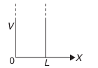
Consider a particle restricted to move along the x-axis between $x = 0$ and $x = L$, by ideally reflecting, infinitely high walls of the infinite potential well, as shown in Fig. Suppose that the potential energy $V$ of the particle is zero inside the box, but rises to infinity outside, that is,

$V(x) = 0$ for $0 \leq x \leq L$ (inside the box)

$V(x) = \infty$ for $x < 0$ and $x > L$ (outside the box)

In this case, the particle is said to be moving in an infinitely deep potential well. To evaluate the wave function $\psi$ in the potential well (where $V = 0$), Schrödinger's equation is written as:

$$\frac{\partial^2 \psi}{\partial x^2} + \frac{8 \pi^2 mE}{h^2}\psi = 0 \quad \text{(i)}$$

By setting $\frac{8 \pi^2 m E}{h^2} = k^2$, the equation becomes:

$$\frac{\partial^2 \psi}{\partial x^2} + k^2 \psi = 0 \quad \text{(ii)}$$

The general solution of this differential equation is:

$$\psi(x) = A \sin kx + B \cos kx \quad \text{(iii)}$$

where $A$ and $B$ are constants.

Applying the boundary condition $\psi(x) = 0$ at $x = 0$, we obtain:

$$A \sin (0) + B \cos (0) = 0 \quad \Rightarrow \quad B = 0$$

With $\psi(x) = 0$ at $x = L$, we have:

$A \sin kL + B \cos kL = 0 \quad \Rightarrow \quad A \sin kL = 0$

This equation is satisfied when:

$$kL = n \pi$$

or

$$k = \frac{n \pi}{L} \quad \text{where} \, n = 1, 2, 3, \ldots$$

or

$$k^2 = \frac{n^2 \pi^2}{L^2} \quad \text{(iv)}$$

or

$$\frac{8 \pi^2 m E}{h^2} = \frac{n^2 \pi^2}{L^2} \quad \text{(v)}$$

or in general we can write Eq. (v) as

$$E_n = \frac{n^2 h^2}{8mL^2} \quad \text{where} \, n = 1, 2, 3, \ldots$$

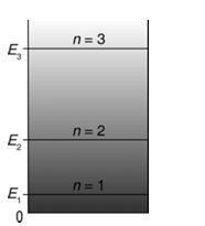
Therefore, in an infinite potential well, the particle cannot have arbitrary energy but only certain discrete energy values corresponding to $n = 1, 2, 3, …$. These are called the eigenvalues of the particle in the well and constitute the energy levels of the system. The integer $n$ corresponding to the energy level $E_n$ is called its quantum number as shown in fig below.

The wave function (or eigen function) is given by Eq. (iii) along with the use of expression for $k$

$$\psi_n(x) = A sin \frac{n \pi x}{L}$$

or

$$\psi_n(x) = A sin kx$$